Lennart's weblog

Notes about open source software, computers, other stuff.

Page 6 of 14

Permantly ban an IP address with fail2ban

Over the last few days I noticed in my logwatch e-mails that one IP address kept trying to log in to my server, even though it was blocked regularly by fail2ban.

Here’s a post that explains how to simply add a list of IP addresses to block permanently. There’s only one catch: the listing provided there contains an error, the word <name> is missing in the iptables command, probably due to HTML conversion. This is the correct line to be insterted into the actionstart section of /etc/fail2ban/action.d/iptables-multiport.conf:

cat /etc/fail2ban/ip.blacklist | while read IP; do iptables -I fail2ban-<name> 1 -s $IP -j DROP; done

Use the following command to check if the IP address is indeed banned:

$ sudo iptables  -L fail2ban-ssh
Chain fail2ban-ssh (1 references)
target     prot opt source               destination         
DROP       all  --  192.168.20.25        anywhere            
RETURN     all  --  anywhere             anywhere 

Related Images:

Replacing a character in a Bash variable name

Today I needed to replace a : in a bunch of file names with a -, so I wanted to write a Bash for-loop to do just that. I vaguely remembered that you can do character replacements within variables, but couldn’t remember the details.

This is how it’s done:

for filename in *; do
    mv "$filename" "${filename/:/-}"
done

I put the variables in double quotes, because the file names contained spaces.

Related Images:

How to start a LaTeX enumerate environment with a different number

I keep forgetting how to do this, so here’s a quick post that shows how to start a LaTeX enumerate environment with a different number.

By default enumerate environments start counting from 1 (obviously). To start with a different number you simply need to change the value of a counter:

\begin{enumerate}
   \setcounter{enumi}{2}
   \item This will be item 3
   \item Item 4 will be here
\end{enumerate}

If you have nested enumerate environments, the counters are enumii and enumiii.

Related Images:

Showing other users (from LDAP) in the LightDM greeter

Ubuntu Linux uses the LightDM greeter (the login screen you see after booting). Since I’m using an LDAP server to store my user accounts and LightDM by default only shows local users I needed to tell LightDM to give me an ‘other user’ option where I can enter a user name and password (I first checked to see if my LDAP connection work by logging in with an LDAP user from the console (tty1).
LightDM is configured in /etc/lightdm/lightdm.conf, but also provides command line tools to set the options. To show the ‘other user’ use:

sudo /usr/lib/lightdm/lightdm-set-defaults --show-manual-login true

This will disable the user list. It adds the line

greeter-show-manual-login=true

to the lightdm.conf file.
If you only want to see the “Other” entry run:

sudo /usr/lib/lightdm/lightdm-set-defaults --hide-users true

And lastly you can turn off guest:

sudo /usr/lib/lightdm/lightdm-set-defaults --allow-guest false

Thanks to mfish at askubuntu.com!

Related Images:

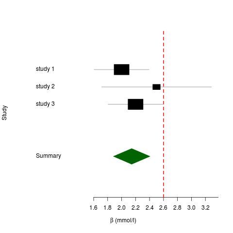
Doing a quick fixed-effects meta-analysis using the Rmeta package

This is a quick example of how to do a fixed meta-analysis using the R package Rmeta, just so I dont have to look it up again next time:

## Create data frame containing betas and standard errors
df <- data.frame()
df <- rbind(df, c(2., 0.2))
df <- rbind(df, c(2.5, 0.4))
df <- rbind(df, c(2.2, 0.2))
 
## Add study names
df <- cbind(df, c("study 1", "study 2", "study 3"))
 
colnames(df) <- c("beta", "se_beta", "name") 
 
## Do the meta-analysis 
ms <- meta.summaries(df$beta, df$se_beta, names=df$name)
 
## Add some colors
mc <- meta.colors(summary="darkgreen", zero="red")
 
## Make a forest plot
plot(ms, xlab=expression(beta ~ " (mmol/l)"), 
     ylab="Study", colors=mc, zero=2.6)

The resulting plot looks like this:
Forest plot of fake data

Related Images:

ProbABEL v0.4.1 released

Last week I released v0.4.1 of ProbABEL, just a few days after releasing v0.4.0, which contained a small, but irritating bug.

This release took quite some time to create, but features quite a few bug fixes, including a major one: for the first time since the filevector format was introduced somewhere in 2009/2010, the Cox proportional hazards regression module works with filevector/DatABEL files. This is a major step forward, because up till now we had to maintain two branches of code: trunk, with all the regular updates and improvements, and the old branch that contained the Cox PH module that was only capable of reading text files.

Another notable change is the incorporation of \chi^2 values in the output files. At the moment these are based on the LRT (likelihood ratio test), except where that doesn’t make sense (e.g. when using the --mmscore option. The implementation was relatively easy, because part of the code was still there from previous versions; it was disabled however, because it didn’t deal with missing genotype data. Now it does. Using the LRT is also easier in the case of the 2df (or genotypic) genetic model, where using the Wald test is not straightforward.

The third user-visible change was a change in the [code]probabel.pl[/code] script that hides some of the details (e.g. the location of the files with genotype data) of running a regression for the user. Previously, using the -o option meant that the output file name was constructed from the name of the phenotype file, the argument of the -o option and a fixed extension that depends on the model(s) being run. Starting with v.0.4.0 this behaviour has changed. If the -o option is specified its argument is used as the start of the output file name, with only the fixed extension appended to it. This allows users to specify output in a different directory than the one where the phenotype file was created.

Packages for Ubuntu Linux (or one of its derivatives and probably also Debian) can be found in the GenABEL PPA (personal package archive). Previously we also released pre-compiled Windows binaries, but I’ve stopped doing that. They were never tested anyway, and I think there isn’t much demand for them anyway. Most people who do genome-wide association studies use Linux servers anyway.

Development of ProbABEL (and other members of the GenABEL suite) takes place on this R-forge page. If you are in search of an open source project to contribute to, feel free to contact us!

User support for the GenABEL suite can be found at our forum.

Related Images:

Using BibTeX from org-mode

I use Emacsorg-mode a lot for writing notes, todo lists, presentations and writing short reports. Recently I started writing a larger report which I normally would have done in LaTeX. This time, since the notes related to the project were already in org format, I decided to write the whole report in org-mode. The one thing I needed for that was using BibTeX bibliographies (and RefTeX) from org-mode. A quick web search revealed that that can easily be done by adding the following to your .emacs file:

;; Configure RefTeX for use with org-mode. At the end of your
;; org-mode file you need to insert your style and bib file:
;; \bibliographystyle{plain}
;; \bibliography{ProbePosition}
;; See http://www.mfasold.net/blog/2009/02/using-emacs-org-mode-to-draft-papers/
(defun org-mode-reftex-setup ()
  (load-library "reftex")
  (and (buffer-file-name)
       (file-exists-p (buffer-file-name))
       (reftex-parse-all))
  (define-key org-mode-map (kbd "C-c )") 'reftex-citation)
  )
(add-hook 'org-mode-hook 'org-mode-reftex-setup)

After that, RefTeX works, but exporting the org document to PDF (via LaTeX) didn’t include the bibliography entries. A quick look at the error log showed that bibtex hadn’t been run, so the question was: how to tell org-mode to do that too when exporting. The answer is to tell org-mode to use the latexmk Perl script (on Debian/Ubuntu it is easily installed from the package repositories) when exporting to PDF. I added the following lines to my .emacs file:

;; Use latexmk for PDF export
(setq org-latex-to-pdf-process (list "latexmk -pdf -bibtex %f"))

Related Images:

Growing XFS and still not able to write files, enough free space

One of the XFS filesystems at work almost ran out of space recently, so I extended the Logical Volume it was on, followed by xfs_growfs. This worked fine, df -h showed enough free space for the upcoming data. In the XFS FAQ I read that by default all inodes are placed in the first 1 TB of disk, which could lead to problem. Therefore, I added the inode64 option to the mount options and ran

mount -o remount

on the partition.

While reviewing my log messages this morning I noticed a lot of

No space left on device

messages for that filesystem. Having this inode64 option in mind I wondered what went wrong. Although df -h and df -i showed enough free space and free inodes, respectively, I still couldn’t create a file. Again the XFS FAQ had an entry for that, but it puzzled me, because I was already using the inode64 option. Since the filesystem wasn’t in use I decided to completely unmount it and then mount it again. That worked. Apparently -o remount is not enough to enable the inode64 option.

Related Images:

Viewing a .bam file in the console

One thing we do regularly at work is taking a look at aligned sequences of human DNA as generated by what is called “next-generation sequencing”. This data is stored in so-called .bam files, which can get pretty large. For example, the .bam file for an individual whose whole genome is sequenced at 12x coverage is approximately 60GB.
To view these files, to check the alignment, look at the coverage of a specific region, etc, people typically use graphical browsers like the IGV or Savant. However, these require you to either run the tool on the server (which means relatively slow X-forwarding over SSH) or copying the BAM file to your local machine, which also takes a lot of time, especially if you want to take a look at a single region for a bunch of people.

For jobs like that I’ve found the text-based viewer integrated in SamTools to be very convenient. It’s a matter of running

samtools tview sample.bam /path/to/reference.genome.fasta

after which you get a view like this:

1000821   1000831   1000841   1000851   1000861   1000871   1000881   1000891   1000901
GGCCAGGCAGGGCTTCTGGGTGGAGTTCAAGGTGCATCCTGACCGCTGTCACCTTCAGACTCTGTCCCCTGGGGCTGGGGCAAGTGCCCGATGGGAGCGCA
.....................................................................................................
..........          ......................A.......................T...............G........A........C
...........                                     .....................................................
............                                           ..............................................
..........................................................C...........      .......................A.
...................................................................................        ..........
                                                                                           ..........

Using g followed by 1:23000000 you will jump to the given position on the given chromosome.
If the 1:23000000 doesn’t work, check the header of the BAM file to see how the chromosome is specified (sometimes it is chr1:23000000, for example):

samtools view -H sample.bam

In the above example the dots indicate nucleotides that are identical to the reference (shown in the second line), the positions with letters indicate reads where a different base was read. In this example all of them are probably sequencing or alignment errors because only one discordant read is observed at any position. If you find a column with letters that means this position is indeed different from the reference. Also notice how the various reads are aligned and that in this case the coverage doesn’t seem to be very high.

Related Images:

Setting up (or fixing) an encrypted swap partition

Today I tried to clone my laptop’s harddrive to a new drive (thanks to Lenovo for sending me a replacement since the old drive was showing signs of breaking down). At first I tried dd, but that failed at around 90%, either because the old disk is indeed failing or because something fishy with the USB connection or enclosure in which I put the new disk. So I started gparted to check which partitions were copied OK and which weren’t. It turns out that all partitions were fine, except for my (encrypted) swap partition. gparted didn’t even recognise the partition type (on the original drive!). So after I replaced the harddrive I wanted to recreate the encrypted swap partition. It turn’s out to be easy if you follow the steps outlined in this blog post from Puny Geek. Thanks Puny Geek!

Related Images:

« Older posts Newer posts »

© 2024 Lennart's weblog

Theme by Anders NorĂ©nUp ↑